How does FTIR work?

The Editor

I receive a steady trickle of enquiries along this line and some of them have been included in Dear Readers [only the ones that have some general interest!]. It is clear from some of the enquiries that many (perhaps most) of you don’t really know how your FTIRs work. Oh I know you’ve all seen the one paragraph description of an interferometer, but very few pieces I have seen tell you how it’s done – what goes on under the cover! Now I’m the sort of idiot who does (or rather ‘used to’) do his own car repairs and I like to know the details. So, I thought I would write a piece for you on this fascinating subject.

The basic idea

The building blocks of an F-T are very different from the predecessor, the double beam (diffraction) infrared spectrometer. In an F-T you have the chain –

Source →Interferometer →Sample →Detector

Each building block varies from manufacturer to manufacturer but basically they all obey the same laws of physics. I can’t be exhaustive, but I will try to cover most of the bits and pieces used in contemporary instruments.

Sources

The easy bit. All the manufacturers use a heated ceramic source. The composition of the ceramic and the method of heating vary but the idea is always the same, the production of a heated emitter operating at as high a temperature as is consistent with a very long life. Historically, people have achieved this objective in almost bizarre ways e.g. using an old fashioned gas mantle, or the Nernst Glower [a device utilising the fact that some ceramics conduct electricity when heated. The Nernst had to be pre-heated and then could be used as a conductor and hence as a hot source – they were tricky to use and unreliable]. These days, the manufacturers tend to go for either a conducting ceramic or a wire heater coated with ceramic. Now, as I explained recently when talking about hot samples in Raman spectroscopy, heated objects emit, the emission occurs at all wavelengths AND the emission at any wavelength increases with temperature. The plots of emission vs. frequency are shown in Figure 1.

Figure 1. Blackbody curves for a variety of temperatures on an absolute wavenumber abscissa scale, (a) in watts, (b) in counts per second. As the temperature is increased the overall intensity increases and the maximum of the curve shifts to higher temperature.

All infrared spectrometers are energy limited i.e. they are short of photons hence it is obvious that the hotter the source, the better. Equally obviously, it would be disastrous if the source operated at a variable temperature so manufacturers go to some lengths to prevent draughts passing the hot source. This is not as easy as it sounds because air will inevitably convect past the source due to its temperature. Many manufacturers get round this problem by monitoring the source output, using the output signal to control the electrical power in a feed-back loop.

Figure 2. The Source emits and is detected by D_S. Output regulates the chip C_D which controls the power fed to the source.

Ideally, then we have a stabilised hot source operating at a feverishly high temperature. Well not quite!

As all you folks who have kept an eye on the atmospheric pollution game will know, heating air to high temperatures can be problematic – generation of the notorious (NO)_x !

The equilibrium N₂ + O₂ ⇌ NO₂ ⇌ N₂O₄ lies overwhelmingly towards the reactants BUT moves towards NO₂ and hence N₂O₄ at elevated temperatures. Unfortunately, as it turns out, good modern sources can be hot enough to generate measurable amounts of NO₂ (and other nitrogen oxides hence (NO)_x). In the atmosphere, this would be only a trivial nuisance, one swamped by other sources of pollution but inside the sealed housing of an FTIR, the (NO)_x can well cause unwanted absorption and even corrosion of the metal and plastic components. So, sources are hot but not too hot. Temperatures vary but a little above 1000º C are fairly typical. Talk of 2000 K is, I suspect, not realistic.

Interferometers

We all know that the interferometer is the heart of our instrument. The interferometer is the bit that analyses the infrared or near infrared and hence enables us to generate a spectrum. Most of us will have at one time or another seen the classical diagram of an interferometer and had it explained to us. Let’s go through this again.

The classic Michelson Interferometer involves a beam splitter – a component which reflects about ½ of the radiation that hits it and transmits the rest. One bundle of radiation follows one path and the remainder a different path. The two bundles are then recombined and pass out of the device. Now, one path is changed in length allowing radiation to interfere with that following the fixed path. In Figure 3, I show the classical diagram of the Michelson Interferometer.

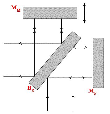
Figure 3.

Parallel radiation entering the device hits beam splitter BS and is either reflected to mirror M_F or transmitted to hit mirror M_M. Radiation reflected by the mirrors then passes either through or is reflected off the beam-splitter and hence either goes back towards the source OR goes forward and out of the interferometer. Thus, only half the radiation entering the interferometer can get out in the OUT direction. Half is reflected back towards the input.

Let’s assume we use monochomatic radiation of wavelength l. If the paths involving M_F and M_M are identical in length, about ½ of the radiation will pass through the interferometer, but if the paths differ by l/₂ when recombined on the beam-splitter, the two bundles of radiation will be out-of-phase and hence cancel each other out. Now, if M_M is moved, the efficiency with which the interferometer will pass radiation follows what is shown in Figure 4.

Figure 4.

If now, we use radiation of 2 wavelengths l₁ and l₂ the result is shown in Figure 5,

Figure 5

that is, we will actually observe the sum of the two cosine functions. If white light is used, we will see the sum of all the cosine functions typical of ALL the wavelengths.

Now, note one feature – at zero path difference all the radiation of whatever wavelength passes through the interferometer. At any other path difference, only some will pass. Hence, the plot of the efficiency of transmissions vs. path difference for white light looks something like

Figure 6.

And is characterised by a “centre burst” at zero path difference and a very complex pattern of waves symmetrically dispersed about it. [Go now to your FTIR and call up the interferogram of the background and you will see a much better picture than the one I have drawn for you in Figure 6].

The interferogram, as Figure 6 is not recognisable as a spectrum. To convert it into something useful, it needs to be Fourier Transformed. At this stage, all textbooks launch into calculus, but I have always found that students went cross-eyed when I tried, so here is a simple-minded explanation of the Fourier Transform process.

Let’s assume the interferogram is digitised and stored in a processor. Now let us also assume that the spectrum we want spans the range 4000 →400 cm^-1 (or in near infrared instruments 12,000 →2,500 cm^-1). If the processor is told to generate a cosine function for radiation frequency 4000 cm^-1 (wavelength 2.5 µ) it can then search the memorised interferogram for its presence to produce a function F. The search can then be made for radiation of frequency 3999 cm^-1 and so on down to 400 cm^-1 . The outcome will be the results shown in Figure 7.

Figure 7. Plot of F vs Frequency in cm^-1

A series of points define how much of the various waveforms are present in the interferogram. Put another way, the FT processor acts as a ‘frequency analzyer’. If the computer is then told to join up the points the result is a recognisable spectrum.

Figure 8.

[Now go to your machine and run a spectrum of anything you like at 4 cm^-1 resolution. Put it up on the screen and then expand the cm^-1 axis. Once very well expanded you will see that indeed the spectrum is a series of straight lines joining points].

Let us leave the transformation here and come back to it later and then also discuss resolution and other details. Let’s look at real instruments first

Practical Interferometers

Early interferometers (and some persist to this day) use a system identical to that in Figure 1. To make the light parallel, mirror collimators (C) are used and so the instrument looks like Figure 9.

Figure 9. A complete Michelson Interferometer.
J= Jacquinot stop, M₁= off-axis ellipsiod,
M₂ & M₃= off-axis paraboloids.
Note the Beamsplitter BS need not be at 45°
to the incoming beam. It rarely is in real instruments,

All components are firmly fixed to a base but mirror M_M moves backward and forwards on an axis normal to its surface. Clearly, the movement must be smooth, reproducible and involve no wobble or shake. These requirements are hard to achieve and lend to the use of high precision engineering. Two solutions are commonly found –

1. Air Bearing Here, a very accurate cylinder houses an equally accurate piston. The latter is ever so slightly smaller than the cylinder and the gap is filled with flowing compressed air. In fact, the piston never touches the cylinder – it floats. A magnetic coil then provides the forward and backward movement. See Figure 10. The air acts as a lubricant but it leaks into the spectrometer. If dry air or N₂is used, no problem, the leaking air purges the interferometer.

Figure 10.

2. Spring Links
   The idea here is to mount the moving mirror on a lattice of thin metal blade springs so that movement is allowed in the required direction and no other. It sounds a bit crude but it works OK. It is hard to get long movements this way and hence the method tends to be confined to the smaller cheaper instruments. See Figure 11.

Figure 11. As usual Mm is the moving mirror, A the armature and C the drive coil. The thin springs are S.
As drawn, the system won’t work. A real system is far too complex to draw (or rather I chickened out!). Can anyone suggest WHY it won’t work? Ed

Whatever method of mirror movement is selected, some shake and wobble is inevitable so some manufacturers have attempted to reduce the problem by using the “corner cube”. Imagine a hollow cube made of mirrors. Now cut it in half across its diagonal. Looking into one of the halves you will see –

The device has a peculiar property very useful to surveyors and instrument manufacturers. Regardless of the angle at which it is held, light entering the corner cube will be reflected accurately back upon itself – less need to establish or maintain precise alignment! Mirror M_M can be replaced by a corner cube and shake and wobble will be much less of a problem than if a plane mirror is used. See below in Figure 12.

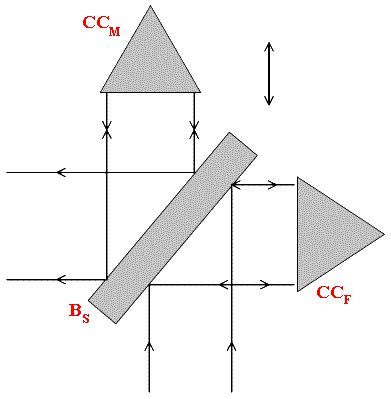
Figure 12.

One manufacturer has eliminated the need to move one mirror completely. They use a system designed to increase and decrease the optical path by rocking an assembly of mirrors about an axis. Such a system is drawn in Figure 13. The problem is that extra reflections are introduced into the optical path but the advantage is that rocking around an axis can be made very precisely and CHEAPLY, shake need not occur and wear is almost non-existent. The rocking mirror assembly is driven by a linear electric motor.

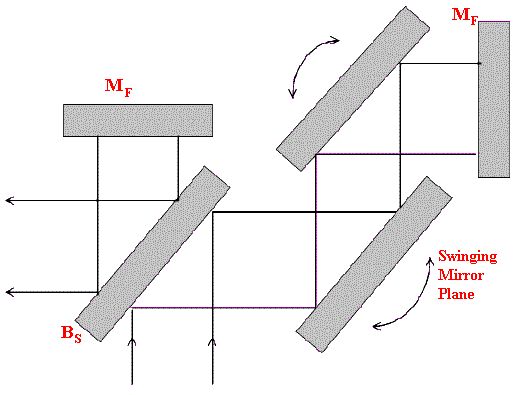
Figure 13

So – we have our interferometer and hence, as we shall see our interferogram. The next problem is to measure the path difference. A ruler is no good, the path difference has to be measured to an accuracy limited only by the precision of the engineering in the interferometer itself. The way this is done is to use the interferometer itself to do the job and to feed it with a source of precisely known wavelength. The He/Ne laser has a wavelength near 632.8nm and is known to very high precision. If a He/Ne laser beam passes through the interferometer, its intensity at the output will generate a superb simple cosine with a peak in intensity every 632.8nm of change in the path difference. How this can be done is shown below in Figure 14.

Figure 14. An example of an early FTIR –
the 1700 Series Perkin Elmer instrument.
J= Jacquinot stop, J₁ is real, J₂ is imaginary.
Both mirros M are fixed

The He/Ne laser generates a parallel beam reflected along the axis of the interferometer by tiny mirror M_L1 . The beam leaving the interferometer is picked up by mirror M_L2 and passed to a detector [or rather 2 detectors. If polarised light is used,(thus polariser P) the interfered radiation is split into two polarisation analysed signals, it is possible for the electronics to work out whether the path difference is increasing or decreasing]. The output of the detector(s) is a cosine. As the signal switches from positive to negative about the mean, a trigger circuit is operated providing a pulse twice every 632.8nm of charge in path difference. As we shall see, this pulse train is in effect used to measure the path difference.

Figure 15. Output from the He/Ne detector
(usually called the fringe detector(s).

In modern instruments, the He/Ne laser beam is moved out of the optic axis of the interferometer so that the infrared beam is not contaminated with red He/Ne radiation. It is usually passed along an optical bath above or below the infrared beam.

The radiation leaving the interferometer is then passed through the sample area before being focussed onto the detector. Figure 16a and b show the optical diagram and schematic of a complete instrument.

Figure 16a.

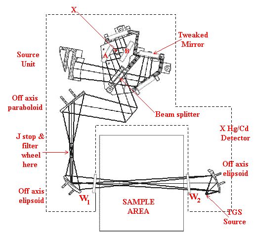
Figure 16b. A modern compact FTIR.
X is the pivot axis of the swinging mirrors A & B.

This is all very well, but how is the interferometer actually aligned ? The job is done roughly at the factory, but in use it needs very frequent optimisation. This is done by tweaking the orientation of the fixed mirror M_M over tiny angles using electric motors or solenoids driven by software. In fact, in some research grade interferometers several ^He/_Ne laser beams are used and the alignment is maintained at perfection continuously.

Detectors

Various detectors are encountered in FTIRs, FTNIRs and F-T Raman instruments. The vast majority act as photo resistors i.e. thay have a very high resistance in the dark and this falls as light falls on them. The most sensitive are the Ge and InGaAs semi-conductor devices. In the dark, they can have resistance as high as 3×10⁸W. Measuring resistance at these high values and doing so rapidly requires the use of very clever electronics if spurious signal (noise) is not to be added to the detected signal. All semi-conductor detectors show an ‘absorption edge’ i.e. they will ignore radiation longer than a characteristic wavelength.

Cooling detectors invariably reduces the amount of noise they develop [we are all familiar with noise. If you listen to your car radio you will be aware that in some areas the sound is clear, in others it is accompanied by hiss – this is “noise” in electronics language. The ratio of signal: noise (S:N) is critical in the measurement of electrical signals and also in the pleasure in listening to your car radio or mobile phone], but unfortunately cooling shifts the absorption edge towards shorter wavelength. Some detectors give adequate performance (an acceptable useful S:N ratio) at room temperature but others must be cooled.

In an FTIR, one normally finds a TGS or similar detector for ordinary use. If better results [or more often, you need results on samples or sample accessories that transmit very little light] are required, one then resorts to the use of a cryogenically cooled mercury cadmium telluride semi-conductor detector. Thus, these are invariably used in infrared microscopy and very often in diffuse reflection experiments.

The output from the detector goes to a preamplifier where it is converted into a voltage signal varying with time. This signal has to be digitised and the job is usually done with a dedicated ‘analogue to digital’ converter chip. These devices will measure the input voltage in binary numbers with 8, 16, 20 or 32 or more digits. Clearly, the number of useful digits is governed by the quality (S:N ratio) of the signal. 16 and 20 bit devices are frequently used.

An A/D converter will carry out the conversion only when it is told to do so – it needs a pulse (or ‘handshake’) to tell it to do the job. The pulse is provided by the He/Ne fringe detector and trigger circuit. So, the A/D converter makes its measurement every 316.4nm of path difference. Clever, ain’t it? Thus, the He/Ne makes it possible to measure the interferogram at ultra precise path difference intervals. If the temperature changes, or you lean on the FTIR, the interferometer will very slightly distort and hence the interferogram will shift. However, the He/Ne beam will ALSO shift helping to correct for the distortion.

The digitised interferogram is now fed to the F-T processor. This can be a dedicated chip or a PC. Obviously, a dedicated chip has its advantages (simplicity, lower cost etc) but the PC increases the versatility enormously. The block diagram looks like Figure 16b.

Operation of FT instruments

Spectroscopists are concerned predominantly about two parameters – signal:noise and resolution. To a lesser extent they worry about time – how long must I scan to get my results? Let’s consider each issue in turn.

Signal:Noise Ratio

Once your instrument has generated a spectrum and put it up on the screen, you will be aware of the S:N ratio. In theory a spectrum should consist of bands (signal) against a smooth background (i.e. N=zero). In reality this is not so, the background varies at random and the peak height jitters up and down (or will vary in height when you measure it again and again). See Figure 17.

Figure 17.

Noise in spectra stops you detecting weak bands and also restricts you in making reliable quantitative measurements [I will write a piece about his in a future edition of IJVS]. You can reduce the noise i.e. enhance the S:N ratio by co-adding scans. The improvement you can achieve is by a factor of n² where ‘n’ is the number of scans. So, the noise in a spectrum can be reduced by a factor of 10 by adding 100 spectra and dividing the summed intensities by 100 [this is the co-addition process]. Many users simply set the instrument to scan once or 4 times or some other “house style”. This isn’t very logical. Some spectra appear against strong backgrounds and tend to be noisier than when the bands stand against a low flat background. I advise setting the instrument to run to the maximum sensible (say 20) scans and that you examine the co-added spectra as they appear on the screen. Once you see what you want – stop the scanning. Now “see what you want” sounds very subjective – very unscientific, but this really is the way we all work. There is no ‘ideal’ or ‘acceptable’ signal:noise ratio. In routine work you know whether a spectrum is good, bad or indifferent [but remember your GOOD may be someone else’s VERY BAD!]

Recording spectra

When you record a spectrum you are, in fact recording two and ratioing them. Let me explain. You empty the sample area (or accessory) and record a BACKGROUND – you then insert the sample, run again and the computer produces a spectrum. What actually happens is that you first record the emission spectrum of source attenuated by the losses in the instrument, the response characteristics of the detector and any absorption along the optical path. The resultant BACKGROUND looks very different from the true emission characteristics of the source. Thus, the beam splitter characteristics and the performance of the detector attenuate the high frequency end of the spectrum. Meanwhile, H₂O+CO₂ in the optical path between the source and the detector cause sharp absorptions
[Run the ‘BACKGROUND’ on your instrument and display it on the screen. You will see intense absorption around 2300 cm^-1 and 670 cm^-1 – these are due to CO₂. The forest of bands around 3200 and 1600 cm^-1 are due to the vibration rotation spectrum of water – for an explanation refer to my piece in Edition 3, Volume 5 earlier this year].

The next spectrum you then record is with the sample in place and again is the emission spectrum of the source, attenuated as before but ALSO by the sample. Usually this is not displayed but rather the second spectrum is immediately ratioed against the first on a point-by-point basis. The result is to show the difference between the two i.e. the spectrum of the sample which is what you want.

Once you understand what happens several sources of possible error become clear –

You can’t get meaningful results if you ratio nothing against nothing! So, if the background emission is non-existent, as it is over the CO₂ absorption near 2300 cm^-1, you get no useful results.

If you record the background under one set of conditions (resolution, number of scans etc) and the spectrum under another, the ratioing will be meaningless. It turns out that if the number of scans in the BACKGROUND is greater than that in the sample spectrum you are OK. You can, however, change the conditions between BACKGROUND and sample spectrum unwittingly.

If you breath into the sample area as you insert the sample you will increase the CO₂ and water vapour in the optical path. As a result, the BACKGROUND you are using is not appropriate and spurious bands will appear in your spectrum. If your instrument is purged with dry nitrogen, opening the sample area will introduce CO₂ + H₂O so the BACKGROUND and sample spectrum must again contain unwanted differences. This article is getting a little long so let me come back to these matters in another piece in a future edition.

Resolution

Like S:N ratio resolution as actually visualised by the user is somewhat subjective. We all have a sort of feel for RESOLUTION – it’s the ability to pick out one band from another lying close to it. So, we want to be sure that if two bands lie xcm^-1 apart we can see them i.e.

Lord Rayleigh way back in the 1800’s defined resolution in terms of the appearance of the spectra but now that we have incredibly monochromatic laser sources people define resolution in terms of ‘bandwidth’. If you take a truly monochromatic source and pass its emission through an instrument you will actually see

The width of the band at exactly ½ of its height is defined as the resolution. The same criteria apply to absorptions – if the absorption is very sharp and almost monochromatic e.g. a vibration rotation band of a gas at a low pressure, the W_½value of the absorption band will be its measured resolution.

The instrument makers offer us resolution values on FTIRs. Do the offered values match what I have said above? Well, the answer is yes and no! The industry accepts a rather different set of criteria to define ‘resolution’. The standard is that the ‘resolution’ is related to the data point density in the Fourier Transformed Spectrum, the standard being that the resolution is ½ the data point density. Let me give you an example -–if you set the resolution at 2cm^-1, the instrument will compute a spectral data point every wavenumber 4000, 3999, 3998 .. 401, 400 cm^-1.

The data points will then be joined up and that’s what you get. The quality of spectrum you actually see depends on the wavenumbers where the data points are calculated and the wavenumber of the emission or absorption bands but the industry standard is reasonable.

So, I hear some of you ask – what resolution should I use? This is a very tricky question to answer: if the absorption band is very sharp – its W_½ is small, you must use better resolution than if it is broad. The general rule is that to avoid missing the details in your spectrum, the resolution value MUST be less than the minimum W_½ value of any bands in your spectrum. In the IR this is a pretty easy criterion to meet because the vast majority of bands are broad (W_½ values >5cm^-1 and sometimes a lot wider than 10cm^-1). In gas phase work, the bands can be incredibly narrow (low- pressure spectra can show W_½ values as low as 0.1cm^-1 routinely). Crystalline materials can sometimes catch you out and have relatively narrow lines but for most purposes 4 cm^-1 resolution is OK for analytical work. If the 4 cm^-1 spectrum looks as if it has fine detail in it – run a 2 cm^-1 spectrum [remember you must use a new 2cm^-1 BACKGROUND!] and see if there is any difference. If not, you can use 4 cm^-1 resolution in future.

One obvious question is – why not record all spectra at the best resolution of which my equipment is capable? The answer is time (or more strictly S:N ratio).

Remember, the resolution is standardised as a half of the data point density – so the number of data points between 4400 and 400cm^-1 will be a modest 2000 at 4 cm^-1 resolution, but will rise to 16,000 at 0.5cm^-1 resolution. To be able to calculate more data points, more points must be measured i.e. the interferogram must be longer. In fact, the way it works out, the length of the interferogram – the distance scanned by the moving mirror equals ¹/_resolution. So – a machine capable of 0.1cm^-1 resolution requires that M_M will move by at least 10 cm, a long way remembering the precision of movement required. This is why small cheap machine tend to offer only restricted resolution.

Recording more data points is all very well, but more time is then needed to calculate the points in the spectrum. To sum up – using a better resolution than is required is simply not worth it because it loses time.

There is also another variable. As resolution is improved and hence the mirror travel increases it becomes essential to restrict the beams that lie off the optical axis of the interferometer. To achieve this – the size of the Jacquinot Stop [JS in Figure 9 and 16b] is reduced as the resolution is improved. Typical values are ~8mm diameter at 4 cm^-1 resolution and perhaps 3mm at 1cm^-1 or less. The effect is that less energy passes through the interferometer when operated at high resolution than at low. To the user this means that more scans are required to achieve an adequate S:N ratio – again soaking up even more time.

To conclude, I have explained the basics of how your FTIR, FTNIR or FT-Raman works but I have said almost nothing about the ruses that you can adopt to fit the experiment to your needs. All instrument makers provide a wide range of software with their most basic instruments, but very few users actually try anything but the most bog standard set-up. This really is a pity.

In the next volume, I will write a piece for you taking you through these features of your instrument showing you what you can do with them.

REF: P.J.Hendra, Int. J. Vib. Spect., [www.irdg.org/ijvs] 5, 5, 2 (2001)